| Last updated: 2008 | |||||||||||||||||||||||||||||
| GNUFOR2 is a module written in Fortran90, which helps to plot graphs/surfaces/histograms/images in Fortran90. It is based on the GNUFOR interface, written by John Burkardt. Here is the main idea of how it works: a Fortran program calls a subroutine (for example call plot(x,y) ) which then creates two files named command_file.txt and data_file.txt. After that GNUPLOT is started automatically via a system command, and it uses commands from the first file and the data from the second to create the plot. After this part is finished, the control is returned to the original Fortran program which called subroutine plot(x,y) (either immediately or after some specified interval of time).
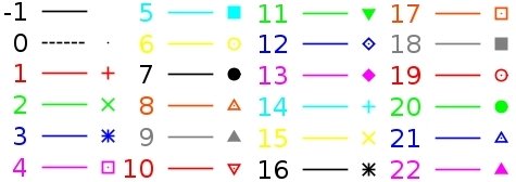
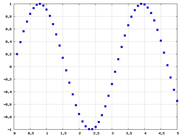
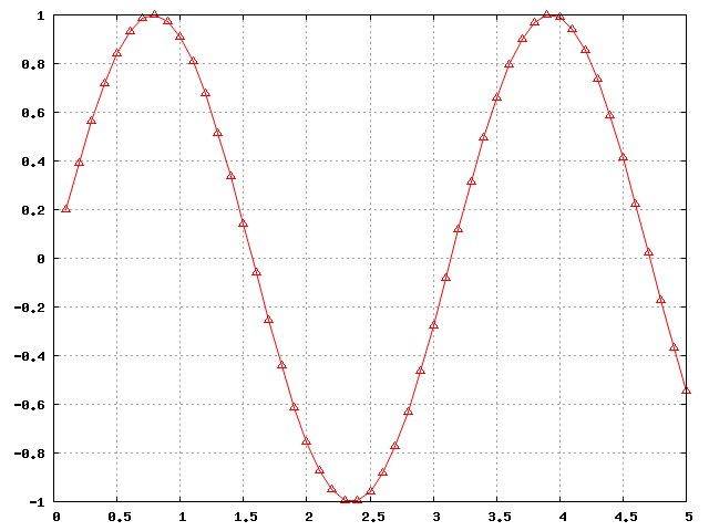
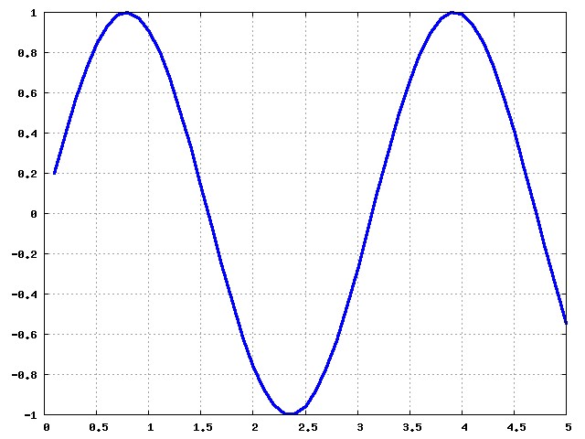
Please note that while this program might be useful for visualising certain data produced by your Fortran program, it can not completely replace Gnuplot. Gnuplot has much more functionality which allows to fine tune almost every detail of the figure. For example, if I want to produce publication quality figures, I would call one of these subroutines from my Fortran program, but then I would edit by hand command_file.txt to obtain the desired results. I would also recommend an excellent program Inkscape for editing pdf (and other vector graphics) files. Here you can find the files: This module was tested under Ubuntu distribution of GNU/Linux, both with GNU Fortran and Intel Fortran compilers. To run the test program, first copy all of the above files into the same folder. Note that the Makefile is written for GNU Fortran, so you have to change the first line in the Makefile if you are using a different Fortran90 compiler. Next, open your favourite shell terminal, navigate to the above mentioned folder, and type: The list of common optional parametersFirst of all, all the subroutines presented below have the following OPTIONAL parameters: pause, terminal, filename, persist, input. Below I explain their meaning. real(kind=4) :: pause -- this parameter is responsible for the delay between the moment the graph is drawn and the moment the control is returned to the program. The default behavior (if you do not specify this parameter) is pause=0. If you set pause=5.3, Gnuplot will finish drawing the graph, wait for 5.3 seconds and then return control back to the original Fortran program. If you set pause equal to ANY NEGATIVE NUMBER ( pause=-1.0 or pause=-3.0), Gnuplot will wait untill you click Enter, and only then pass the control back to Fortran program. character(len=*) :: terminal -- this parameter is responsible for the output format. The default terminal is 'wxt' -- the interactive window created by the wxWidgets library. The 'terminal' parameter is most useful if you want to save the picture as a file. Some possibilities are character(len=*) :: filename -- the output is saved to a file with this name. The default filename has the format 'date-hours-minutes-seconds-milliseconds'. This format is useful in the situation when you are creating many pictures in a loop, and you want to save all of them (of course with different filenames so that they do not overwrite each other). The downside of this default setting is that the filename changes every time you run a program, and soon your folder will be littered with lots of files. Setting filename='my_file' will always save the figure into the same file. Note that this option only has effect when the terminal is set to 'ps', 'jpeg','png' or something similar - it is useless if the figure is not being saved into a file. character(len=*) :: persist -- this is an important parameter. The default is persist='yes', which means that the window with the graph will NOT be closed after the Fortran program has finished executing. However, this can become a problem if you are creating many graphs in a loop, since you will end up with dozens (maybe hundreds) of Gnuplot windows on your Desktop. This can be easily changed, if you set persist='no' in the parameter list. This parameter is usually used together with pause parameter. For example: character(len=*) :: input -- this parameter is only important for an interactive terminal 'wxt'. The default behavior is that commands and data are always saved into files with names 'command_file.txt' and 'data_file.txt'. This might be a problem when you are creating several graphs which persist after the Fortran program has finished executing.The above two files might be overwritten, and you won't be able to explore the graph using the interactive tools of 'wxt' terminal. Here is when 'input' parameter becomes useful: you can specify different file_names for each graph. For example, if you set input='f1', the above two files will be named 'command_file_f1.txt' and 'data_file_f1.txt'. The list of main subroutines and their parameterssubroutine plot(x1, y1, style, pause, color1, terminal, filename, polar, persist, input, linewidth)The only mandatory parameters are two arrays x1(:), y1(:) ot type real(kind=8). They must have the same size. character(len=3), optional :: style -- this parameter is responsible for the linestyle. By default the graph is drawn with lines. You can change this by specifying: IMPORTANT: Note that there is a space in front of 5 in the previous example. The style parameter for each graph must have length equal to three. Thus if point type is a double digit number, you would just type style='xx-'. But if the point type is a single digit number, you must type a space in front of this number style=' x.' so that the length is still equal to three. Different point types:
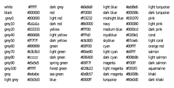
character(len=*), optional :: color1 -- the color of the lines/points. You can specify the color by giving its name color1='dark-blue', or by giving it's RGB value color1='#334455'. Here is the list of colors recognizable by Gnuplot :
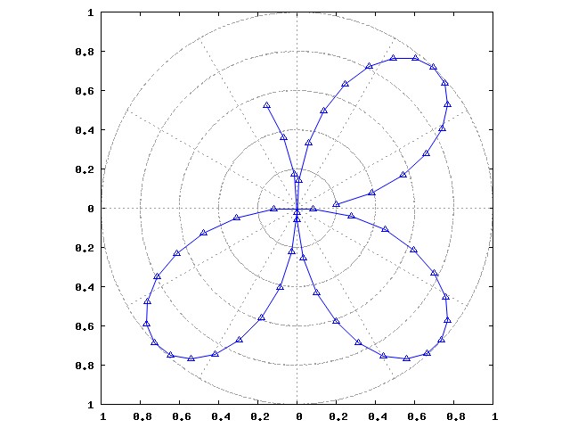
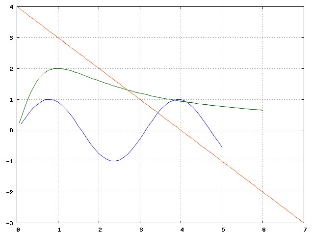
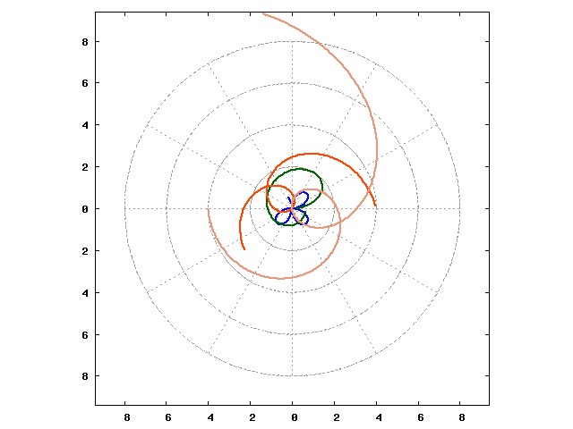
real(kind=4), optional :: linewidth The default is linewidth=1.0, you can change it to any real (positive) value. character(len=*), optional :: polar -- switch to polar coordinates by setting polar='yes'. Examples:call plot(x1, y1)
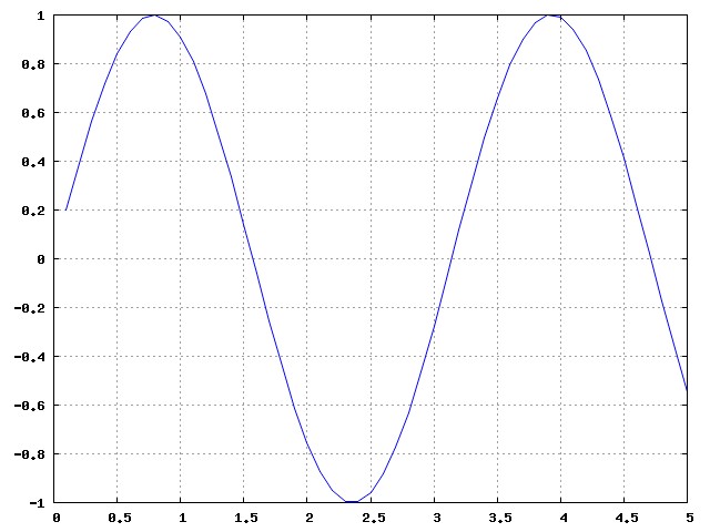
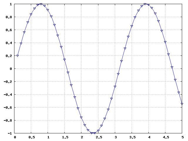
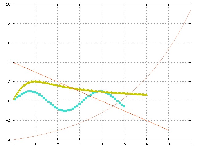
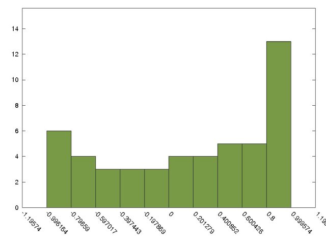
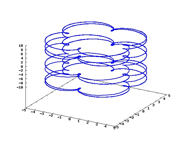
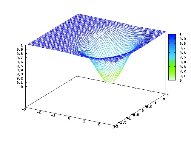
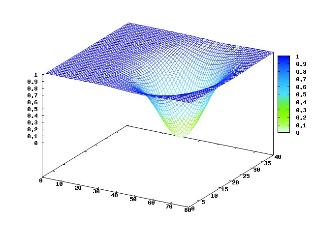
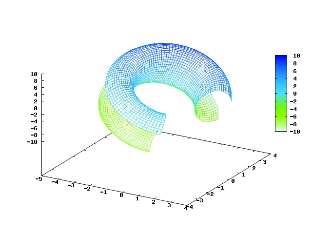
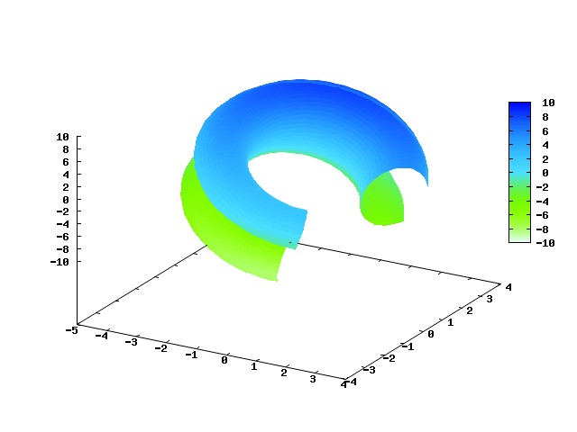
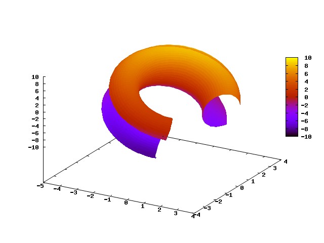
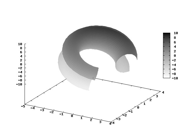
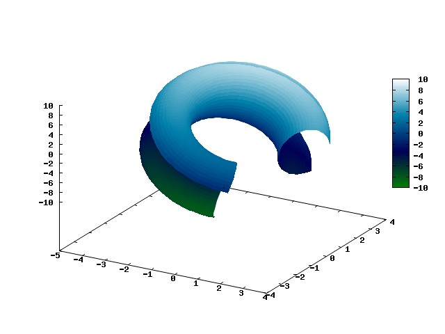
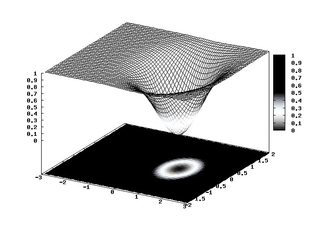
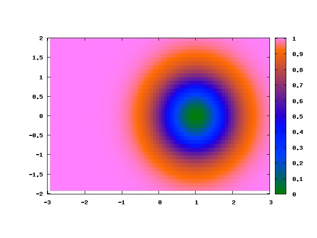
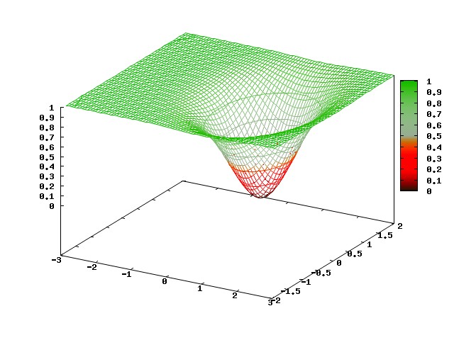
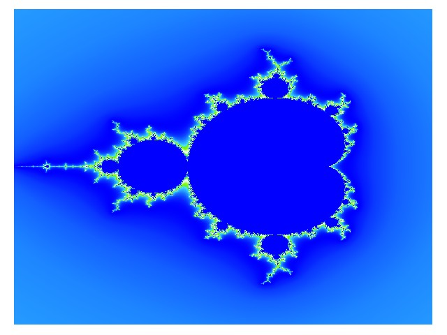
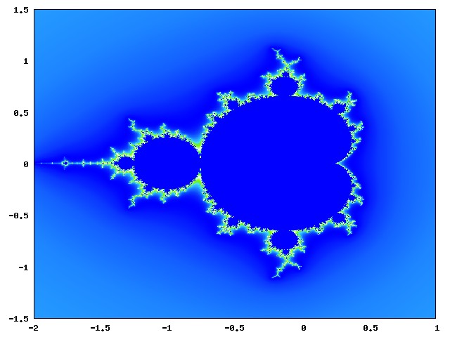
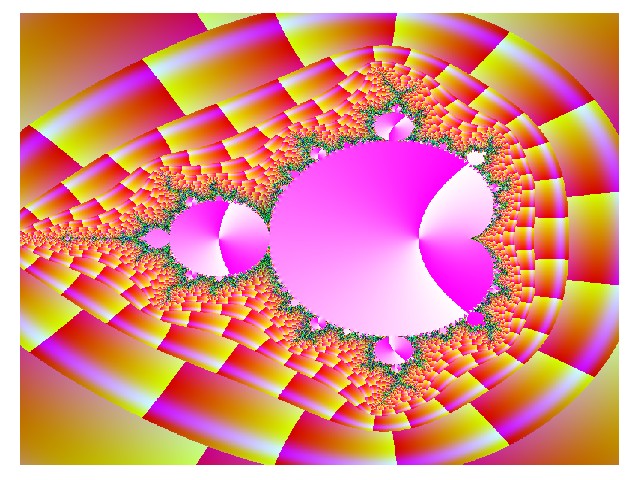
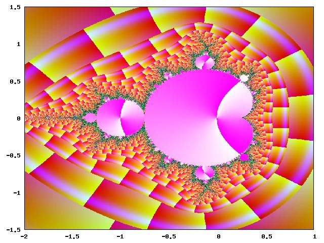
call plot(x1, y1, pause=0.5) call plot(x1, y1, pause=0.5, persist='no') call plot(x1, y1, '20-', color1='#886622', polar='yes') call plot(x1, y1, x2, y2, x3, y3, linewidth=3.0) call plot(x1, y1, x2, y2, x3, y3, x4, y4, ' 5.10- 0. 7-', color2='magenta', filename='my_picture', terminal='ps') -- note that in this case the length of style parameter must be 12 = 3 characters X 4 plots.subroutine plot3d(x, y, z, pause, color, terminal, filename, persist, input, linewidth)This is a subroutine for plotting curves in 3D. The mandatory parameters are real(kind=8) arrays x(:), y(:) and z(:) of the same size. The remaining parameters are optional, and have the same meaning as for subroutine 'plot'. Note that the style parameter is absent, also only one plot per window is possible.subroutine hist(x, n, pause, color, terminal, filename, persist, input) This a simple subroutine for plotting histograms. The mandatory parameters are real(kind=8) array x(:) (the data) and an integer value n - the number of bins. The other optional parameters have the same meaning as before. subroutine surf(z(:,:), pause, palette, terminal, filename, pm3d, contour, persist, input) These subroutines create a surface plot in 3D. The first two are useful for creating plots of surfaces given by z=z(:,:)=f(x,y), while the third subroutine is useful for creating plots of parametric surfaces: character(len=*), optional :: palette You can choose from the list of predefined pallettes (RGB, HSV, CMY, YIQ or XYZ) or you can specify your own. The default value is CMY . These are some of the examples: character(len=*), optional :: pm3d -- this parameter specifies the use of the pm3d algorithm. Possible uses include: character(len=*), optional :: contour -- this parameter specifies the behavior of contour plot. Possible uses include: subroutine image(gray(:,:), pause, palette, terminal, filename, persist, input) These subroutines plot the matrix as an image: each matrix element is taken as a color. The mandatory parameters for the first subroutine is real(kind=4) square matrix of positive numbers gray(:,:) which represent intensity at each pixel. The second subroutine takes as input an integer array rgb(:,:,:), where rgb(1,i,j) represents intensity of red color at pixel (i,j), rgb(2,i,j) is responsible for green and rgb(3,i,j) for blue. IMPORTANT: all the values of rgb(:,:,:) must be integer numbers lying in the interval [0,255]. The first two subroutines just plot the image and do not care about x and y axes. If you want to specify x-y axes, you should use the third and the fourth subroutines. Note that arrays should have compatible lengths: size(x)=size(gray(:,1)) and size(y)=size(gray(1,:)) with similar conditions for rgb(:,:,:). The optional parameters pause, palette, terminal, filename, persist, input have the same meaning as before (see 'surf' subroutine). Note that if you want to draw an rgb image, you do not need to specify the palette parameter, as it would have no effect on the result. The above four subroutines have one drawback - the data_file can be quite large. For example, if you want to produce a 1000x1000 image, the size of data_file.txt is around 25Mb, for 2000x2000 image the file size increases to 100Mb, and so on. Using .rgb files instead of ASCII should decrease the file size. Thus if you know how to produce an .rgb binary file with Fortran -- please email me your suggestions. Examples of the use of subroutines These examples are taken from the program test.f90 (can be found in this archive).See the discussion above on how to compile and run this program. Below each graph you can see the corresponding command.
|


Keele, Glendon and Markham Campus
Contact
(416) 736-2100
Campus Maps